Test Selection | Parametric vs Non-Parametric | Interpretation
- T-test: Compares means between 2 groups. Assumes normality, equal variance, independence.
- ANOVA: Compares means across 3 or more groups. Post-hoc tests needed to identify which groups differ.
- Chi-square: Tests association between categorical variables. Expected count should be over 5 in each cell.
- Regression: Models relationship between outcome and predictor(s). Linear for continuous outcomes, logistic for binary.
- Parametric vs Non-Parametric: Parametric assumes normal distribution (t-test, ANOVA). Non-parametric does not (Mann-Whitney, Kruskal-Wallis).
- “Use paired t-test for before-after comparisons, independent t-test for separate groups
- “ANOVA tells you IF groups differ, not WHICH groups - need post-hoc tests (Tukey, Bonferroni)
- “Fisher exact test preferred over chi-square when expected counts under 5
- “Correlation does NOT imply causation - confounders may explain association
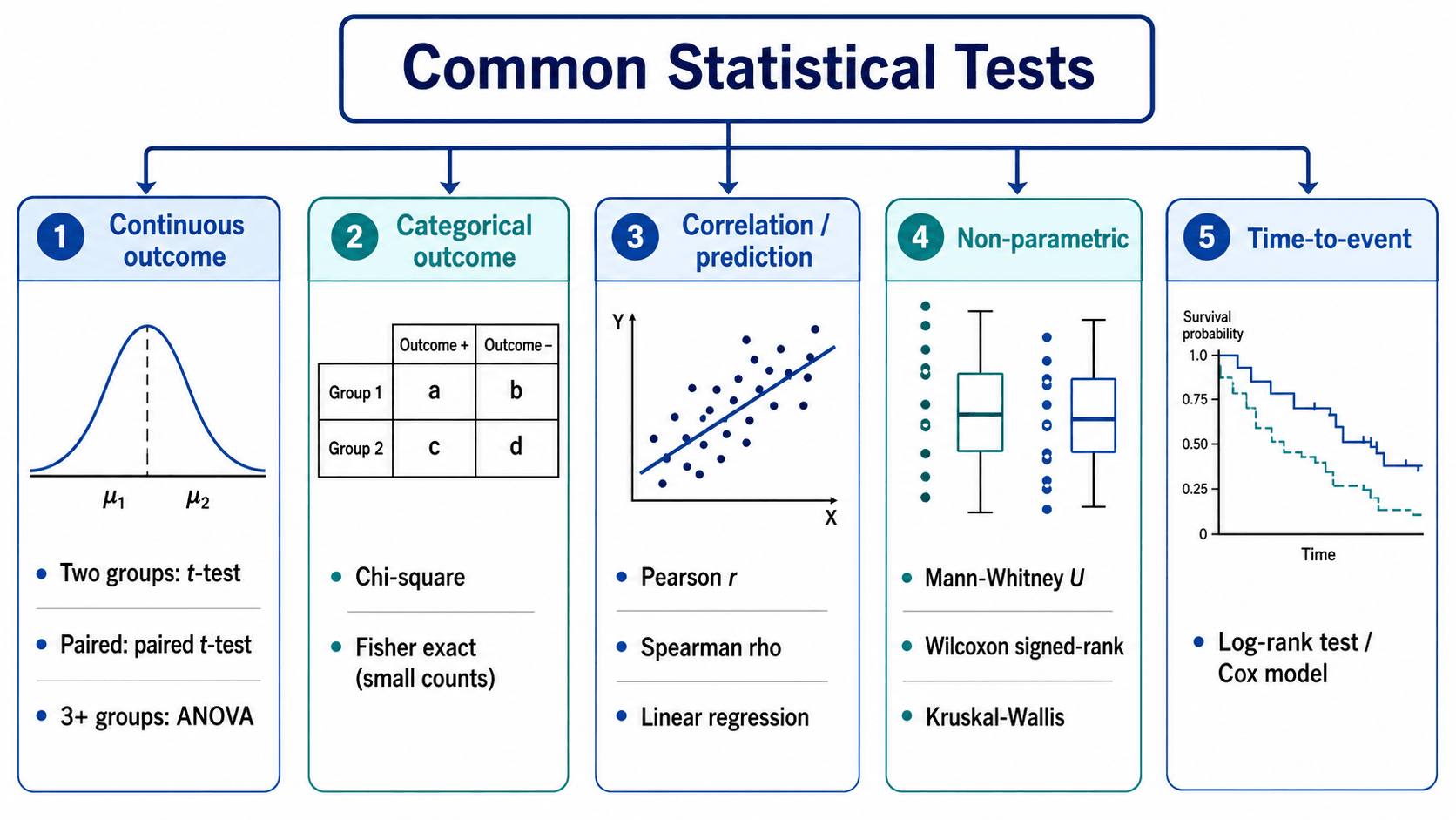
Continuous outcome: t-test, ANOVA, regression. Categorical outcome: Chi-square, Fisher exact, logistic regression. Always match test to data type.
Requirements: Normal distribution, equal variance, independence. Check normality: Histogram, Q-Q plot, Shapiro-Wilk test. If violated: Use non-parametric alternative.
Paired: Same subjects measured twice (before-after). Use paired t-test. Independent: Different subjects in each group. Use independent t-test. Test choice depends on design.
Problem: Testing many groups inflates Type I error. Solution: Use ANOVA first (omnibus test), then post-hoc with correction (Tukey, Bonferroni). Do NOT run multiple t-tests.
Overview and Introduction
Statistical tests are the foundation of evidence-based orthopaedics. Understanding when to use each test and how to interpret results is essential for critically appraising literature and conducting research. This topic covers the most common statistical tests used in orthopaedic research.
Concepts and Mechanisms
Fundamental Statistical Concepts
Hypothesis Testing Framework
- Null hypothesis (H0): Assumes no difference or no effect between groups
- Alternative hypothesis (H1): States there IS a difference or effect
- Type I error (α): Rejecting H0 when it's true (false positive) - typically set at 0.05
- Type II error (β): Failing to reject H0 when it's false (false negative)
- Power (1-β): Probability of detecting a true effect - aim for over 80%
Central Limit Theorem As sample size increases, the sampling distribution of the mean approaches a normal distribution, regardless of the population distribution. This is why parametric tests work with large samples even when data is skewed.
Parametric vs Non-Parametric Tests
- Parametric
- Normality, equal variance
- Non-Parametric
- No distribution assumptions
- Parametric
- Higher when assumptions met
- Non-Parametric
- Lower but more robust
- Parametric
- t-test
- Non-Parametric
- Mann-Whitney U
Effect Size vs Statistical Significance
- p-value: Probability of observing result if null hypothesis is true
- Effect size: Magnitude of the difference (Cohen's d, odds ratio)
- Clinical significance: Whether the effect matters clinically
- A statistically significant result may not be clinically meaningful!
Anatomy of Statistical Tests
Components of a Statistical Test
- t-statistic (t-tests)
- F-statistic (ANOVA)
- Chi-square statistic (χ²)
- Z-score (large samples)
- Larger absolute values = more extreme result
- Compared against critical value or used to calculate p-value
- t-test: df = n₁ + n₂ - 2
- Paired t-test: df = n - 1
- Chi-square: df = (rows-1) × (columns-1)
- ANOVA: df between groups, df within groups
- Affects critical value threshold
- More df = narrower confidence intervals
- p less than 0.05: conventionally "significant"
- p less than 0.01: highly significant
- p less than 0.001: very highly significant
- NOT probability that null is true
- NOT probability that result is due to chance
- 95% CI: 95% confidence true value is within range
- If 95% CI excludes null value → significant at p less than 0.05
- Width indicates precision
- Shows magnitude and precision
- Aids clinical interpretation
Understanding these components allows proper interpretation of statistical test results.
Classification
Classification of Statistical Tests
- 2 Groups (Independent)
- Independent t-test
- 2 Groups (Paired)
- Paired t-test
- 3+ Groups
- One-way ANOVA
- 2 Groups (Independent)
- Mann-Whitney U
- 2 Groups (Paired)
- Wilcoxon signed-rank
- 3+ Groups
- Kruskal-Wallis
- 2 Groups (Independent)
- Chi-square or Fisher
- 2 Groups (Paired)
- McNemar test
- 3+ Groups
- Chi-square
- 2 Groups (Independent)
- Mann-Whitney U
- 2 Groups (Paired)
- Wilcoxon signed-rank
- 3+ Groups
- Kruskal-Wallis
- 2 Groups (Independent)
- Log-rank test
- 2 Groups (Paired)
- N/A
- 3+ Groups
- Log-rank test
Parametric vs Non-Parametric Classification
- Independent samples t-test
- Paired t-test
- One-way ANOVA
- Two-way ANOVA
- Pearson correlation
- Linear regression
- Continuous data
- Normal distribution (or large n)
- Equal variance across groups
- Mann-Whitney U (rank-sum)
- Wilcoxon signed-rank
- Kruskal-Wallis (H test)
- Friedman test
- Spearman correlation
- Ordinal data
- Small sample sizes
- Skewed distributions
- Outliers present
Proper test classification ensures appropriate test selection for your research question.
Diagnostic Test Statistics
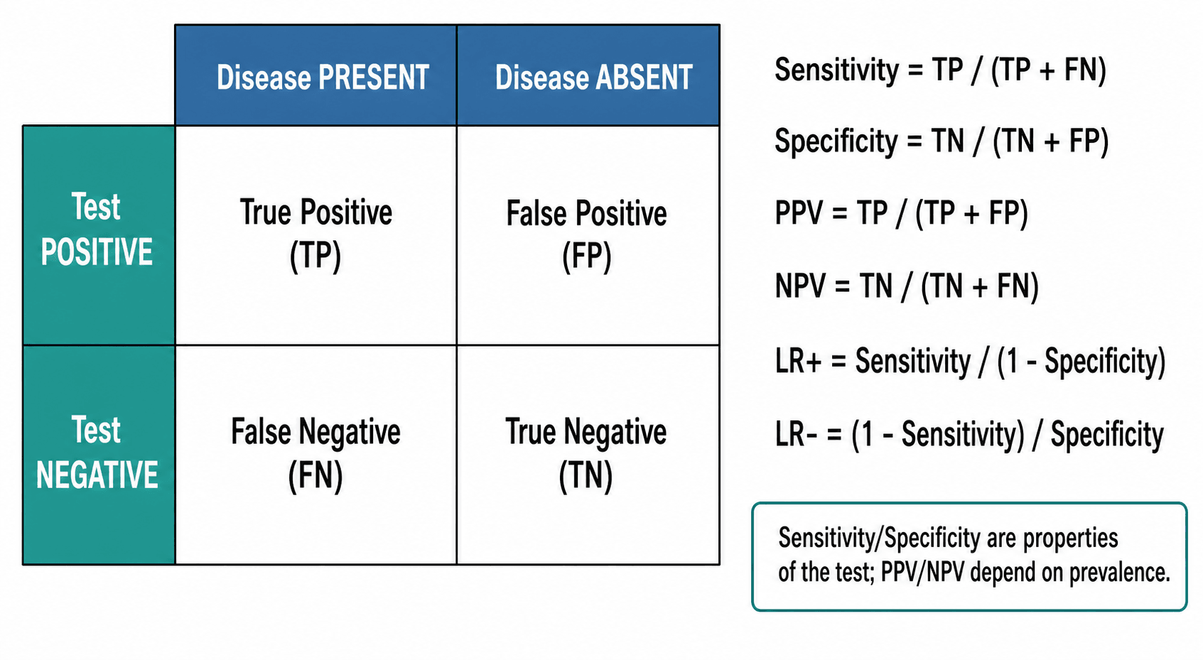
Evaluating Diagnostic Tests
- Proportion of diseased correctly identified
- Formula: TP / (TP + FN)
- High sensitivity = few false negatives
- "Rules OUT disease when negative" (SnNOut)
If sensitivity = 95%, 5% of cases will be missed
- Proportion of non-diseased correctly identified
- Formula: TN / (TN + FP)
- High specificity = few false positives
- "Rules IN disease when positive" (SpPIn)
If specificity = 90%, 10% will be false alarms
- Formula: TP / (TP + FP)
- Depends on disease prevalence
- Higher PPV with higher prevalence
"My patient tested positive - how likely are they to actually have it?"
- Formula: TN / (TN + FN)
- Also depends on prevalence
- Higher NPV with lower prevalence
"My patient tested negative - how confident am I they're disease-free?"
- Disease Present
- True Positive (TP)
- Disease Absent
- False Positive (FP)
- Column 4
- PPV = TP/(TP+FP)
- Disease Present
- False Negative (FN)
- Disease Absent
- True Negative (TN)
- Column 4
- NPV = TN/(TN+FN)
- Disease Present
- Sens = TP/(TP+FN)
- Disease Absent
- Spec = TN/(TN+FP)
- Column 4
Diagnostic test statistics are essential for evaluating imaging studies and clinical tests.
Performing Statistical Analysis
Step-by-Step Analysis Workflow
- Formulate null and alternative hypotheses
- Identify outcome variable(s)
- Identify predictor/exposure variable(s)
- Determine comparison type (difference, association, prediction)
- Check data type (continuous, categorical, ordinal)
- Assess distribution (histogram, Q-Q plot)
- Identify outliers and missing data
- Check for data entry errors
- Use DINGO mnemonic
- Match test to data type and design
- Choose parametric or non-parametric
- Consider confounders (multivariable analysis)
- Normality (Shapiro-Wilk, Q-Q plot)
- Equal variance (Levene test)
- Independence of observations
- Sample size adequacy
- Run analysis in software (SPSS, R, Stata)
- Report test statistic, df, p-value
- Include effect size and confidence interval
- Present results clearly (tables, figures)
Software Options
- Cost
- Expensive
- Learning Curve
- Easy
- Best For
- Beginners, basic analyses
- Cost
- Free
- Learning Curve
- Steep
- Best For
- Advanced users, custom analyses
- Cost
- Moderate
- Learning Curve
- Moderate
- Best For
- Epidemiology, panel data
- Cost
- Common
- Learning Curve
- Easy
- Best For
- Simple calculations only
- Cost
- Expensive
- Learning Curve
- Steep
- Best For
- Clinical trials, pharma
Following a systematic approach ensures rigorous and reproducible statistical analysis.
Practical Examples in Orthopaedics
Common Orthopaedic Research Scenarios
Cemented vs uncemented THA outcomes
Harris Hip Score (continuous, 0-100) Test: Independent samples t-test If non-normal: Mann-Whitney U test
"Mean HHS was 85.2 (SD 12.1) in cemented vs 87.4 (SD 11.8) in uncemented group (t=-1.42, df=98, p=0.16)"
Knee ROM before vs after TKA
ROM in degrees (continuous) Design: Same patients at 2 time points Test: Paired t-test If non-normal: Wilcoxon signed-rank test
"ROM improved from 92° (SD 18) to 115° (SD 12), mean difference 23° (95% CI: 18-28, p less than 0.001)"
Pain scores across 4 fracture types
VAS pain score (continuous) Groups: 4 fracture classifications Test: One-way ANOVA Post-hoc: Tukey or Bonferroni correction
"Significant difference in VAS between groups (F=5.23, df=3,96, p=0.002). Post-hoc: Type D higher than Types A,B (p less than 0.05)"
Smoking status and nonunion rate
Nonunion yes/no (categorical) Exposure: Smoker/non-smoker (categorical) Test: Chi-square test (or Fisher exact if expected less than 5)
"Nonunion rate was 15% in smokers vs 5% in non-smokers (χ²=6.8, df=1, p=0.009)"
These examples demonstrate common statistical scenarios in orthopaedic research.
Common Errors and Pitfalls
Statistical Errors to Avoid
Rejecting null hypothesis when it is true
- Multiple comparisons without correction
- P-hacking (testing until p less than 0.05)
- Selective outcome reporting
- Pre-specify primary outcome
- Use Bonferroni or FDR correction for multiple tests
- Register study protocol before data collection
Failing to reject null when it is false
- Underpowered study (sample too small)
- High variability in data
- Small true effect size
- Conduct a priori power calculation
- Aim for power greater than 80%
- Use sensitive outcome measures
- Using t-test when ANOVA needed (multiple comparisons)
- Using parametric test with skewed data
- Using independent test when data is paired
- Using chi-square when expected counts less than 5
- Follow decision tree (DINGO mnemonic)
- Check assumptions before analysis
- Consult statistician if unsure
- Biased p-values
- Invalid confidence intervals
- Unreliable conclusions
- Normality (Q-Q plot, Shapiro-Wilk)
- Equal variance (Levene test)
- Independence (study design)
- Adequate sample size
Differential: Commonly Confused Tests
- Tempting (Wrong) Choice
- Several independent t-tests
- Correct Choice
- One-way ANOVA then post-hoc
- Discriminator
- Multiple t-tests inflate family-wise Type I error
- Tempting (Wrong) Choice
- Independent t-test
- Correct Choice
- Paired t-test (or Wilcoxon signed-rank)
- Discriminator
- Data are paired, so within-subject correlation must be used
- Tempting (Wrong) Choice
- Pearson chi-square
- Correct Choice
- Fisher exact test
- Discriminator
- Chi-square approximation fails with low expected counts
- Tempting (Wrong) Choice
- Chi-square
- Correct Choice
- McNemar test
- Discriminator
- Chi-square assumes independent observations
- Tempting (Wrong) Choice
- Linear regression
- Correct Choice
- Logistic regression (odds ratios)
- Discriminator
- Linear regression can predict probabilities outside 0-1
- Tempting (Wrong) Choice
- Chi-square on revised vs not
- Correct Choice
- Kaplan-Meier + log-rank / Cox
- Discriminator
- Ignoring censoring and follow-up time biases estimates
- Tempting (Wrong) Choice
- Pearson correlation
- Correct Choice
- Spearman correlation (rho)
- Discriminator
- Pearson assumes linear, bivariate-normal data
Awareness of these errors helps avoid common statistical mistakes.
Reporting and Publishing Results
Reporting Statistical Results
- Report participant flow diagram
- State sample size calculation
- Report all outcomes - primary and secondary
- Include confidence intervals for main results
- Report actual p-values (not just p less than 0.05)
- Intention-to-treat analysis
- Report losses to follow-up
- Baseline characteristics table
- Clear statement of study design
- Describe setting, dates, eligibility
- Report numbers at each stage
- Report outcome data with denominators
- Address confounding
- Case-control, cohort, cross-sectional clearly stated
- Bias assessment
- Sensitivity analyses
Presenting Statistical Results
- Reporting Format
- Mean (SD) or median (IQR)
- Example
- Pain score: 3.2 (SD 1.4)
- Reporting Format
- n (%) with denominator
- Example
- 23/50 (46%) achieved union
- Reporting Format
- RR or OR with 95% CI
- Example
- RR 0.65 (95% CI 0.48-0.88)
- Reporting Format
- HR with 95% CI, survival curve
- Example
- HR 0.72 (95% CI 0.55-0.94)
- Reporting Format
- Exact value to 2-3 decimal places
- Example
- p = 0.034 (not p less than 0.05)
FRACS Viva Point: "What must be reported alongside any p-value?" Answer: The effect size (difference between groups) and 95% confidence interval - p-values alone do not indicate clinical importance or precision of the estimate.
Proper statistical reporting enables readers to evaluate findings and enables future meta-analyses.
Tests for Continuous Outcomes
Comparing Two Groups
Independent Samples t-test
Use When:
- Comparing means between 2 independent groups
- Continuous outcome variable
- Data approximately normally distributed
- Equal variance between groups
Example: Comparing WOMAC scores between cemented vs uncemented THA groups.
Null Hypothesis: Mean outcome is equal in both groups.
Assumptions:
- Normal distribution in each group
- Independence of observations
- Equal variance (homoscedasticity)
Interpretation: p less than 0.05 indicates significant difference in means.
Alternatives if Assumptions Violated:
- Non-normal distribution: Mann-Whitney U test (non-parametric)
- Unequal variance: Welch t-test (does not assume equal variance)
The independent t-test is the most common test in orthopaedic research.
Comparing Three or More Groups
One-Way ANOVA
Use When:
- Comparing means across 3 or more independent groups
- Continuous outcome
- Data approximately normally distributed
- Equal variance across groups
Example: Comparing functional scores across 3 surgical approaches.
Null Hypothesis: All group means are equal.
Key Point: ANOVA tells you IF any groups differ, NOT which specific groups differ.
Post-Hoc Tests (if ANOVA significant):
- Tukey HSD: Compares all pairwise combinations, controls family-wise error
- Bonferroni: Conservative, divides alpha by number of comparisons
- Dunnett: Compares all groups to control group only
Assumptions:
- Normal distribution in each group
- Independence of observations
- Equal variance (homoscedasticity)
Alternative if Violated: Kruskal-Wallis test (non-parametric ANOVA).
Never run multiple independent t-tests instead of ANOVA - inflates Type I error.
Tests for Categorical Outcomes
Chi-Square Test
Use When:
- Comparing proportions between 2 or more groups
- Categorical outcome
- Independent observations
Example: Comparing complication rates (yes/no) across 3 surgical techniques.
Null Hypothesis: No association between variables (proportions are equal across groups).
Requirement: Expected count greater than 5 in each cell of contingency table.
- If violated: Use Fisher exact test (exact p-value, no expected count requirement).
Chi-Square Interpretation
- When to Use
- Expected count greater than 5 in all cells
- Advantage
- Faster, widely available
- Limitation
- Inaccurate with small sample or low expected counts
- When to Use
- ANY sample size, especially expected count under 5
- Advantage
- Exact p-value, no assumptions about expected counts
- Limitation
- Computationally intensive for large tables
Clinical Example: Comparing infection rates (categorical outcome) between smokers and non-smokers.
Understanding when to use chi-square vs Fisher exact prevents incorrect p-values.
McNemar Test (Paired Categorical Data)
The classification and differential tables name the McNemar test as the correct choice for paired binary data - but chi-square and Fisher (above) are for independent groups, so paired categorical data need a different test.
Use When:
- Binary outcome (yes/no) measured on the same subjects twice (before-after), or in matched pairs
- The 2x2 table cross-tabulates the paired responses, not two independent groups
Example: Whether a clinical sign is present before vs after an intervention in the same patients; or whether a finding is positive under two paired test conditions.
How it works: McNemar tests only the discordant pairs - the subjects who changed (yes-to-no and no-to-yes). Concordant pairs (no change) carry no information about change and are ignored; the test asks whether the two directions of change are equally likely.
Why not chi-square: A standard chi-square assumes independent observations, so using it on paired data ignores the within-subject correlation and gives an invalid p-value. For paired categorical data with more than two categories the extension is the Stuart-Maxwell test; for quantifying paired agreement (rather than testing change) use Cohen's kappa (in the reliability table).
McNemar is to chi-square what the paired t-test is to the independent t-test - the paired-data version.
Tests for Associations and Relationships
Correlation
Use When: Assessing strength and direction of relationship between 2 continuous variables.
Pearson Correlation (r)
Use When:
- Both variables continuous
- Linear relationship
- Bivariate normal distribution
Range: r = -1 to +1
- r = +1: Perfect positive correlation
- r = 0: No correlation
- r = -1: Perfect negative correlation
Interpretation:
- r = 0.0 to 0.3: Weak correlation
- r = 0.3 to 0.7: Moderate correlation
- r = 0.7 to 1.0: Strong correlation
Example: Correlation between age and functional score after THA.
Key Point: Correlation does NOT imply causation - confounders may explain association.
Pearson correlation is the most common for linear relationships.
Regression
Linear Regression
Use When:
- Modeling relationship between continuous outcome and predictor(s)
- Predicting outcome value based on predictors
Simple Linear Regression: 1 predictor
- Equation: Y = a + b×X
- b (slope): Change in Y for 1-unit increase in X
Multiple Linear Regression: 2 or more predictors
- Equation: Y = a + b₁×X₁ + b₂×X₂ + ...
- Adjusts for confounders: Each coefficient is adjusted for other variables
Example: Predicting functional score based on age, BMI, comorbidities.
Assumptions:
- Linear relationship
- Normal distribution of residuals
- Homoscedasticity (constant variance of residuals)
- Independence of observations
Interpretation: Coefficient represents change in outcome per unit change in predictor.
Multiple regression allows adjustment for confounders in observational studies.
Test Selection Guide
- Number of Groups
- 2 groups
- Paired or Independent
- Independent
- Test
- Independent t-test
- Number of Groups
- 2 groups
- Paired or Independent
- Paired
- Test
- Paired t-test
- Number of Groups
- 2 groups
- Paired or Independent
- Independent
- Test
- Mann-Whitney U test
- Number of Groups
- 2 groups
- Paired or Independent
- Paired
- Test
- Wilcoxon signed-rank test
- Number of Groups
- 3+ groups
- Paired or Independent
- Independent
- Test
- One-way ANOVA
- Number of Groups
- 3+ groups
- Paired or Independent
- Repeated measures
- Test
- Repeated measures ANOVA
- Number of Groups
- 3+ groups
- Paired or Independent
- Independent
- Test
- Kruskal-Wallis test
- Number of Groups
- 2+ groups
- Paired or Independent
- Independent
- Test
- Chi-square or Fisher exact
Interpreting Research Outcomes
Statistical vs Clinical Significance
P-value less than chosen alpha (usually 0.05)
- The difference is unlikely due to chance alone
- Nothing about magnitude or clinical importance
- Large samples can detect trivial differences
- "Statistically significant" ≠ "important"
- p = 0.04 is not much different from p = 0.06
Difference is large enough to change practice
- Minimal Clinically Important Difference
- Patient-centered threshold
- Varies by outcome measure
- VAS pain: 2 points (or 30% change)
- WOMAC: 15 points
- SF-36 Physical: 5 points
Key Outcome Measures
- Definition
- Risk in exposed / Risk in unexposed
- Interpretation
- RR = 2.0 means double the risk
- Definition
- Odds in cases / Odds in controls
- Interpretation
- Approximates RR when outcome rare (less than 10%)
- Definition
- Control rate - Treatment rate
- Interpretation
- Actual percentage point reduction
- Definition
- 1 / ARR
- Interpretation
- Patients to treat to prevent 1 event
- Definition
- Instantaneous risk ratio over time
- Interpretation
- HR = 0.7 means 30% reduction in hazard
FRACS Viva Question: "A drug reduces DVT risk from 4% to 2%. What is the NNT?" Answer: ARR = 4% - 2% = 2% = 0.02. NNT = 1/0.02 = 50. You need to treat 50 patients to prevent one DVT.
Understanding both statistical and clinical significance is essential for evidence-based practice.
Clinical Applications
Understanding statistical tests allows clinicians to critically appraise orthopaedic literature and make evidence-based decisions. Key applications include:
- Evaluating treatment outcomes: Comparing surgical vs conservative management
- Assessing prognostic factors: Identifying predictors of complications
- Quality improvement: Analyzing registry data for benchmarking
- Research design: Selecting appropriate tests for study protocols
Guidelines, Registries & Global Practice
Global Reporting Standards (Side by Side)
Statistical reporting is governed by internationally harmonised, study-design-specific guidelines endorsed by the EQUATOR Network. These apply regardless of jurisdiction and are referenced by AAOS, NICE, BOA/BOOS, EFORT and most journals.
- Study Design
- Randomised controlled trials
- Key Statistical Mandates
- Pre-specified primary outcome, sample-size calculation, effect size with 95% CI, ITT analysis, flow diagram
- Endorsement
- ICMJE, AAOS/JBJS, BJJ, NICE
- Study Design
- Cohort, case-control, cross-sectional
- Key Statistical Mandates
- Confounder handling, effect estimates with CI, numbers at each stage, sensitivity analyses
- Endorsement
- ICMJE, EFORT, BJJ
- Study Design
- Diagnostic accuracy studies
- Key Statistical Mandates
- Sensitivity/specificity with CI, 2x2 data, ROC/AUC, reference standard
- Endorsement
- Radiology and diagnostic journals
- Study Design
- Systematic reviews and meta-analyses
- Key Statistical Mandates
- Pooled effect with CI, heterogeneity (I-squared), risk-of-bias, GRADE certainty
- Endorsement
- Cochrane, ICMJE
- Study Design
- Prediction/risk models
- Key Statistical Mandates
- Events per variable, calibration, discrimination (C-statistic), internal/external validation
- Endorsement
- Methodology and registry journals
Major Joint Replacement Registries (Global)
- Country/Region
- Australia
- Primary Statistical Output
- Cumulative percent revision (Kaplan-Meier), HR via Cox
- Note
- Near-complete capture, validated revision linkage
- Country/Region
- England, Wales, NI, IoM
- Primary Statistical Output
- Revision rates, PROMs linkage, funnel plots
- Note
- One of the largest registries worldwide
- Country/Region
- Sweden
- Primary Statistical Output
- Implant survivorship, competing-risk analysis
- Note
- Oldest hip registry (from 1979)
- Country/Region
- Norway
- Primary Statistical Output
- Cox regression with adjustment, revision endpoints
- Note
- Strong methodological output
- Country/Region
- United States
- Primary Statistical Output
- Revision burden, cumulative incidence
- Note
- Rapidly growing voluntary registry
Registry follow-up is censored and varies between patients, so a crude revision percentage is misleading. Registries report cumulative percent revision via Kaplan-Meier (or cumulative incidence with competing-risk methods, since death precludes revision) and compare implants with Cox proportional-hazards models adjusted for age, sex and diagnosis. According to PubMed, observational/registry estimates can closely match RCT estimates when confounding is well controlled (Concato et al, NEJM 2000, DOI).
Practice Variation in Statistical Standards
- Significance threshold: p less than 0.05 remains the global convention, but many statisticians (and the American Statistical Association) caution against dichotomising results; some fields advocate reporting exact p-values, confidence intervals and effect sizes instead of a binary "significant/not significant".
- Trial registration: ANZCTR (Australia/NZ), ClinicalTrials.gov (US/international) and ISRCTN/EU-CTR (Europe) all satisfy the ICMJE prospective-registration requirement.
- Fragility of the evidence base: According to PubMed, the median Fragility Index of orthopaedic sports-surgery RCTs is only 2 (Khan et al, AJSM 2016, DOI), so reliance on single small trials varies and meta-analysis is often required.
Australian Research Framework
- National Statement on Ethical Conduct in Human Research
- Mandatory ethics approval for human research
- Australian Code for Responsible Conduct of Research
- Human Research Ethics Committee (HREC) approval
- Informed consent documentation
- Data management plans
- Reporting adverse events
- www.anzctr.org.au
- Mandatory for clinical trials
- Required before participant enrollment
- ICMJE requirement for publication
- Primary and secondary outcomes
- Sample size calculation
- Statistical analysis plan
Australian Orthopaedic Data Sources
- Type
- Registry
- Application
- Joint replacement outcomes nationally
- Type
- Quality standards
- Application
- Clinical care standards, indicators
- Type
- Health statistics
- Application
- National injury and disease data
- Type
- Registry
- Application
- Victoria, NSW trauma outcomes
FRACS Viva Point: "What is the level of evidence of AOANJRR data?" Answer: Level III (retrospective cohort) - but with very high validity due to near-complete capture (greater than 98%) and validated data linkage for revision endpoints.
Australian trainees should be familiar with national research infrastructure and ethics requirements.
MCQ Practice Points
Q: Why should you NOT run multiple independent t-tests when comparing 3 or more groups? A: Inflates Type I error rate. Each t-test has 5% false positive risk. Three t-tests (Group 1 vs 2, 1 vs 3, 2 vs 3) inflate family-wise error to approximately 14%. ANOVA controls overall Type I error at 5%, then post-hoc tests with correction identify specific differences.
Q: When would you use a paired t-test instead of an independent t-test? A: When comparing same subjects at two time points (e.g., before vs after surgery). Paired t-test accounts for within-subject correlation and is more powerful. Independent t-test is for comparing two separate groups of different subjects.
Q: When should you use Fisher exact test instead of chi-square? A: When expected count is under 5 in any cell of the contingency table. Chi-square approximation is inaccurate with small expected counts. Fisher exact provides exact p-value for any sample size.
Q: How do you interpret the Pearson correlation coefficient r = 0.7? A: Strong positive linear relationship. r = 0.7 means 49% of variance in one variable is explained by the other (r² = 0.49). Clinical significance depends on context. Interpretation: r under 0.3 = weak, 0.3-0.7 = moderate, over 0.7 = strong. Note: correlation does not imply causation.
Q: How do you decide between parametric and non-parametric tests? A: Use non-parametric tests when: (1) data violate normality assumption (check with Shapiro-Wilk test), (2) ordinal data (e.g., Likert scales), (3) small sample size where normality cannot be verified, (4) extreme outliers present. Non-parametric tests are more robust but less powerful.
At a Glance
Statistical test selection depends on data type and study design: t-test compares means between 2 groups (paired for before-after, independent for separate groups), ANOVA compares 3+ groups (requires post-hoc tests like Tukey/Bonferroni to identify which differ), chi-square tests associations between categorical variables (use Fisher exact when expected counts under 5), and regression models relationships between outcomes and predictors. Parametric tests (t-test, ANOVA) assume normal distribution—if violated, use non-parametric alternatives (Mann-Whitney U, Kruskal-Wallis). Key pitfall: running multiple t-tests inflates Type I error; use ANOVA first as an omnibus test. Correlation does not imply causation—confounders may explain observed associations.
DINGOChoosing the Right Test
Hook:Follow the DINGO trail to find the right statistical test for your data!
NINEParametric Test Assumptions
Hook:Check NINE assumptions before using parametric tests - or use non-parametric alternatives!
Exam Viva Scenarios
Practise clinical reasoning and management decisions out loud
“You are comparing functional scores between 3 different surgical approaches for rotator cuff repair. What statistical test would you use and why?”
“A study used logistic regression to identify predictors of nonunion after tibial fracture. Age had an odds ratio of 1.5 (95% CI 1.2 to 1.9, p = 0.001). What does this mean?”
Tests for Continuous Outcomes
- 2 groups, independent, normal = Independent t-test
- 2 groups, paired (before-after), normal = Paired t-test
- 2 groups, independent, non-normal = Mann-Whitney U
- 2 groups, paired, non-normal = Wilcoxon signed-rank
- 3+ groups, independent, normal = One-way ANOVA + post-hoc
- 3+ groups, repeated measures, normal = Repeated measures ANOVA
- 3+ groups, independent, non-normal = Kruskal-Wallis
Tests for Categorical Outcomes
- Comparing proportions, expected count over 5 = Chi-square
- Comparing proportions, expected count under 5 = Fisher exact
- Binary outcome with predictors = Logistic regression
- Multiple categorical outcomes = Chi-square or multinomial regression
Tests for Associations
- Correlation between 2 continuous, normal = Pearson correlation (r)
- Correlation between 2 variables, non-normal or ordinal = Spearman correlation (rho)
- Predicting continuous outcome from predictors = Linear regression
- Predicting binary outcome from predictors = Logistic regression (OR)
- Correlation does NOT imply causation - confounders may explain
Critical Test Selection Rules
- Match test to outcome type (continuous vs categorical)
- Check normality before parametric tests (histogram, Q-Q plot, Shapiro-Wilk)
- Use paired tests for before-after, independent for separate groups
- ANOVA first for 3+ groups, then post-hoc (never multiple t-tests)
- Fisher exact when expected count under 5 (not chi-square)
Interpretation Principles
- ANOVA tells IF groups differ, post-hoc tells WHICH groups
- Pearson r: 0-0.3 weak, 0.3-0.7 moderate, 0.7-1.0 strong correlation
- Logistic regression OR greater than 1 = increased odds, OR less than 1 = decreased odds
- Regression coefficients are adjusted for other variables in model
- Non-parametric tests less powerful but more robust to violations
Common Mistakes
- Multiple t-tests instead of ANOVA (inflates Type I error)
- Independent t-test for paired data (loses power)
- Chi-square with expected count under 5 (inaccurate p-value)
- Not checking parametric assumptions before using t-test or ANOVA
- Confusing correlation with causation (observational data)
Evidence Base
P-values Unduly Influence Perceived Importance of Study Results
- Orthopaedic residents, fellows and surgeons rated importance of 40 published studies with and without p-values
- Of 40 comparative studies, 30 reported p less than 0.05 for the primary comparison
- Mean importance scores were higher when a significant p-value was shown (difference 0.6 on a 1-3 scale, 95% CI 0.1 to 1.1)
- 10 of 12 reviewers perceived results as more important when a significant p-value was presented
- Statistically significant p-values exert undue influence on perceived clinical importance
Number of Events Per Variable in Logistic Regression (the 10-EPV rule)
- Monte Carlo simulation of a 673-patient cardiac cohort with 252 deaths and 7 predictors
- Tested events per variable (EPV) of 2, 5, 10, 15, 20 and 25
- For EPV of 10 or greater, regression coefficients showed no major bias or coverage problems
- For EPV less than 10, coefficients were biased in both directions, variance estimates were unreliable, and paradoxical (wrong-direction) associations increased
- Established the widely used minimum of approximately 10 events per candidate variable
Fragility of Statistically Significant Findings in Sports Surgery RCTs
- Systematic survey of 48 RCTs in sports medicine and arthroscopic surgery (2005-2015)
- Median sample size 64 (IQR 48.5-89.5); median total outcome events 19 (IQR 10-27)
- Median Fragility Index was 2 (IQR 1-2.8)
- Changing the outcome status of just 2 patients in one arm reversed significance in the typical trial
- Most statistically significant orthopaedic RCTs are statistically fragile
RCTs, Observational Studies and the Hierarchy of Research Designs
- Compared meta-analyses of RCTs with meta-analyses of cohort/case-control studies on the same 5 clinical topics (99 reports)
- Average summary estimates from well-designed observational studies were remarkably similar to those of RCTs
- Example: BCG vaccine RR 0.49 (95% CI 0.34-0.70) from 13 RCTs vs OR 0.50 (95% CI 0.39-0.65) from 10 case-control studies
- Point estimates were actually more variable across RCTs than across observational studies
- Well-designed observational studies did not systematically overestimate treatment effects
STROBE Statement: Reporting of Observational Studies (Explanation and Elaboration)
- Consensus reporting guideline for cohort, case-control and cross-sectional studies
- 22-item checklist covering title, abstract, introduction, methods, results and discussion
- 18 items common to all designs; 4 items specific to each design
- Explicitly addresses confounding, bias, effect-size reporting and study-flow numbers
- Now required or recommended by most major orthopaedic and medical journals
Quality of Reporting of Confounding in Observational Intervention Studies
- Systematic review of 174 observational intervention studies in 10 general medical and epidemiological journals (2004-2007)
- Over 98% acknowledged the potential for confounding bias
- Only 51% reported details on inclusion of observed confounders and only 10% on their selection
- Just 9% commented on the likely effect of residual (unobserved) confounding
- Median overall reporting quality score was only 4 of 8, with no improvement across years