Diagnostic Test Statistics
- Sensitivity/specificity are calculated DOWN the columns; PPV/NPV ACROSS the rows. Computing sensitivity across a row (the commonest 2×2 error) gives you PPV by mistake.
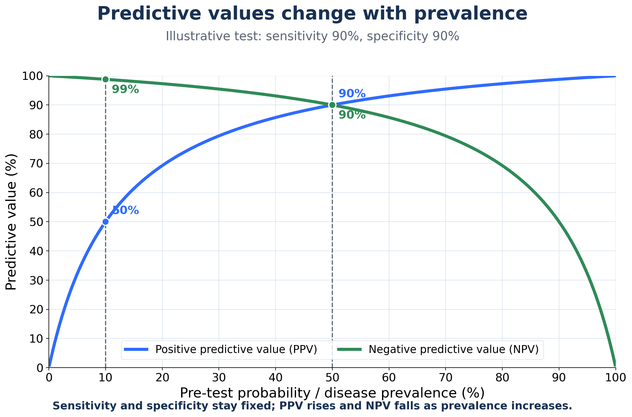
- PPV and NPV depend on PREVALENCE; sensitivity and specificity do not (materially). Quoting a study's PPV for your own population without considering its prevalence is the classic appraisal error - PPV collapses in low-prevalence screening.
- SnNout / SpPin: a Snsitive test, when Negative, rules out; a Specific test, when Positive, rules in. Don't invert them.
- Likelihood ratios are prevalence-INDEPENDENT - that is their advantage over predictive values. LR+ = Sn/(1−Sp), LR− = (1−Sn)/Sp; combine as pre-test odds × LR = post-test odds (not probabilities directly).
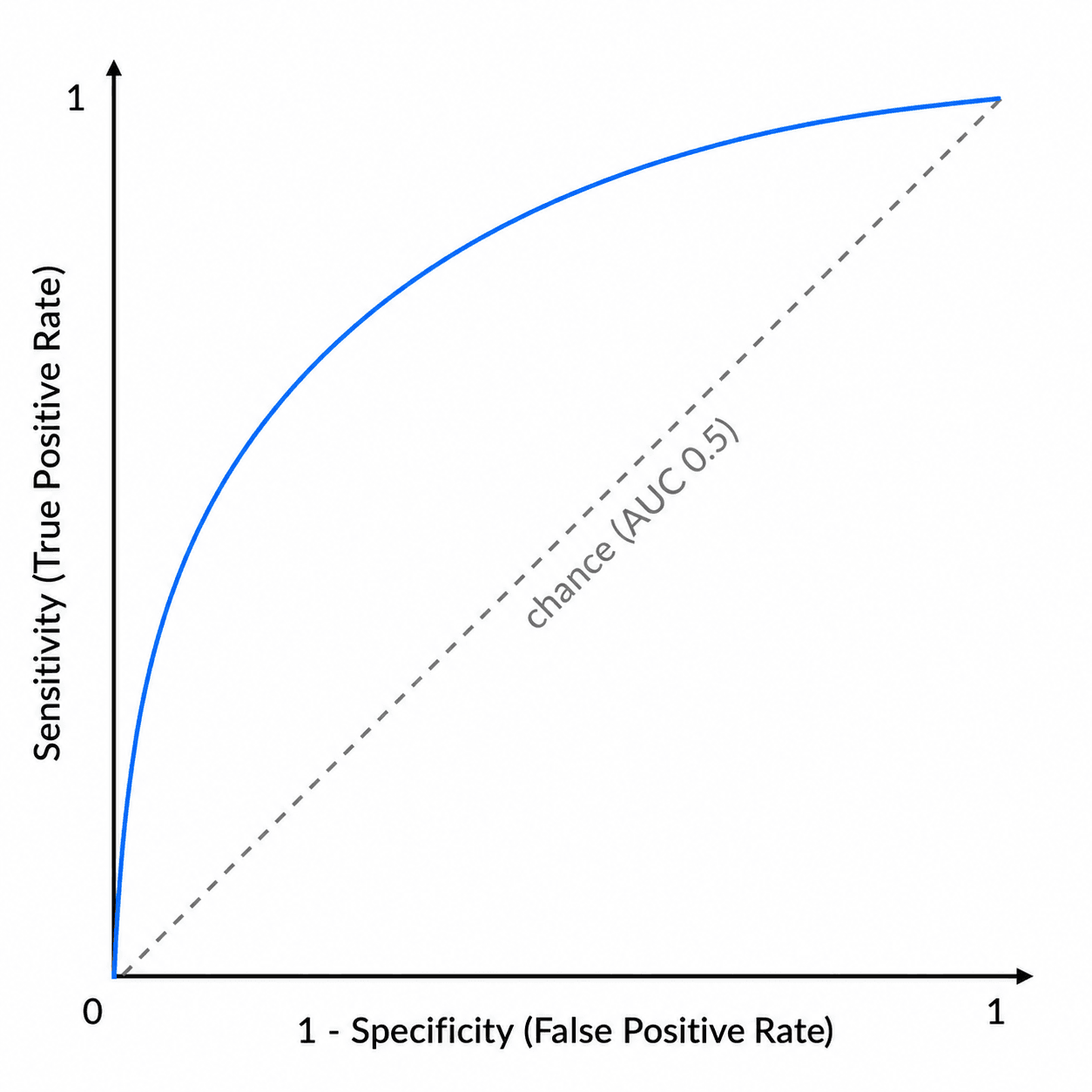
- The ROC plots sensitivity vs (1 − specificity) - not specificity. AUC 0.5 = chance, 1.0 = perfect.
- A high AUC does not mean the test is useful at every threshold - you still pick an operating point by the relative cost of a missed case vs a false alarm.
Overview & Introduction
Diagnostic-test statistics are core evidence-based-medicine / critical-appraisal material - the examiner wants to see that you can take a published test (or your own clinical sign) and say how good it is, and how to apply it to the patient in front of you. Orthopaedics is full of diagnostic tests - the Lachman and pivot-shift for the ACL, the Ottawa rules, the Thompson test, MRI for a meniscal tear - and every one of them has a sensitivity, a specificity and a behaviour that changes with the population.
- It is pure reasoning, not memory - given a 2×2 table you can derive every metric, which is why examiners love it.
- It exposes a common error: confusing test properties (sensitivity/specificity) with the patient's answer (PPV/NPV) and ignoring prevalence.
- It is clinically real: choosing a screening vs a confirmatory test, and interpreting an MRI or a clinical sign, both rest on these numbers.
- The robust numbers (likelihood ratios, AUC) are exactly what a thoughtful candidate quotes instead of a prevalence-bound PPV.
Concepts: the 2×2 table & core formulas
Every diagnostic statistic is built from a 2×2 table comparing the test result against the reference (gold) standard:
- Disease PRESENT
- True Positive (TP)
- Disease ABSENT
- False Positive (FP)
- Row total
- TP + FP → PPV
- Disease PRESENT
- False Negative (FN)
- Disease ABSENT
- True Negative (TN)
- Row total
- FN + TN → NPV
- Disease PRESENT
- TP + FN (all diseased)
- Disease ABSENT
- FP + TN (all well)
- Row total
- N
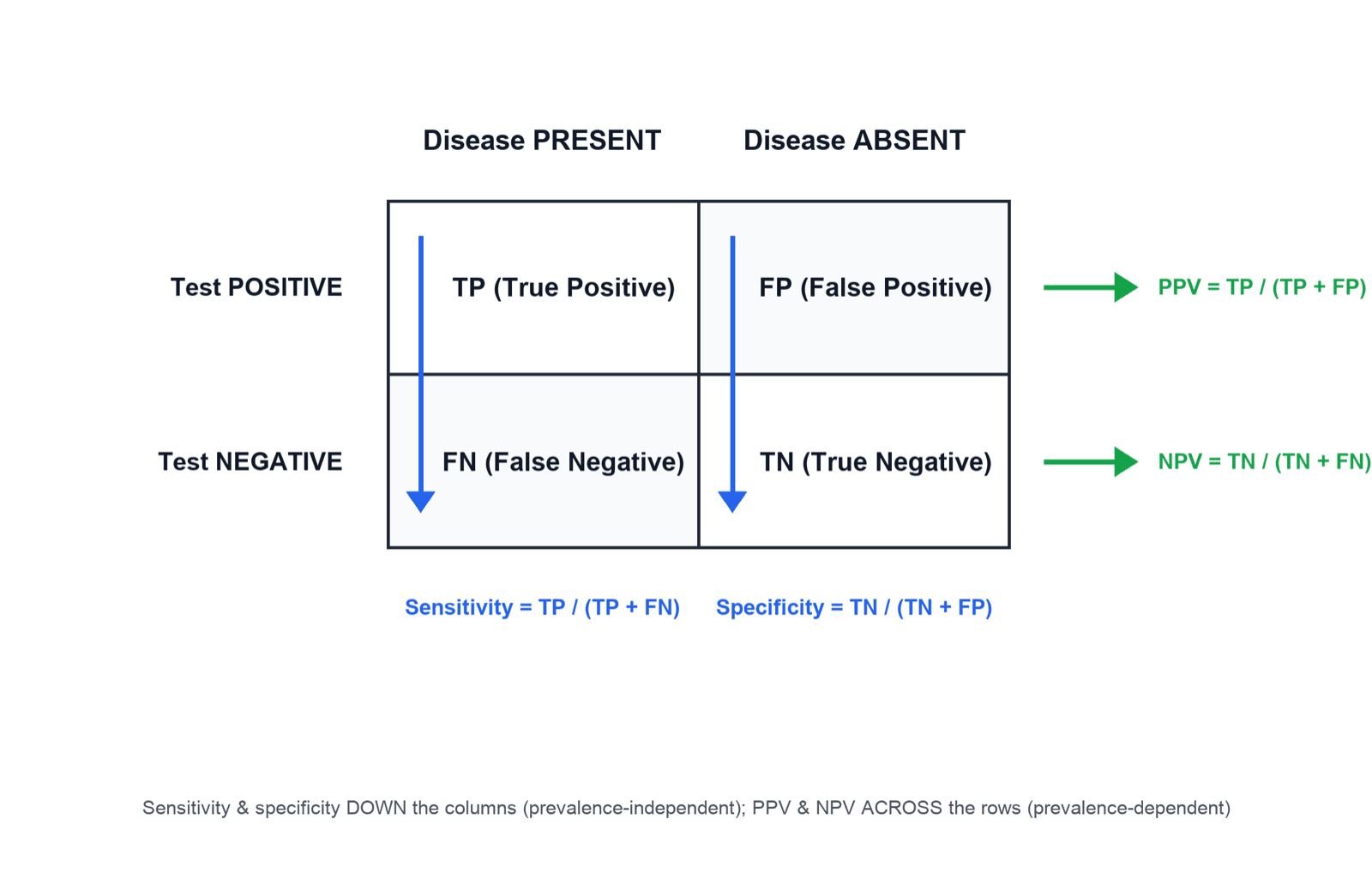
- Sensitivity = TP / (TP + FN) — of all who HAVE the disease, the fraction the test catches (down the "disease present" column).
- Specificity = TN / (TN + FP) — of all who do NOT have the disease, the fraction the test clears (down the "disease absent" column).
- Positive predictive value (PPV) = TP / (TP + FP) — of all who test POSITIVE, the fraction truly diseased (across the "test positive" row).
- Negative predictive value (NPV) = TN / (TN + FN) — of all who test NEGATIVE, the fraction truly well (across the "test negative" row).
Sensitivity and specificity are calculated DOWN the columns (within each true-disease column) — they describe the test and are largely prevalence-independent. PPV and NPV are calculated ACROSS the rows (within each test-result row) — they answer the patient's question but depend on prevalence, so they are population-specific.
Sensitivity & specificity (SnNout / SpPin)
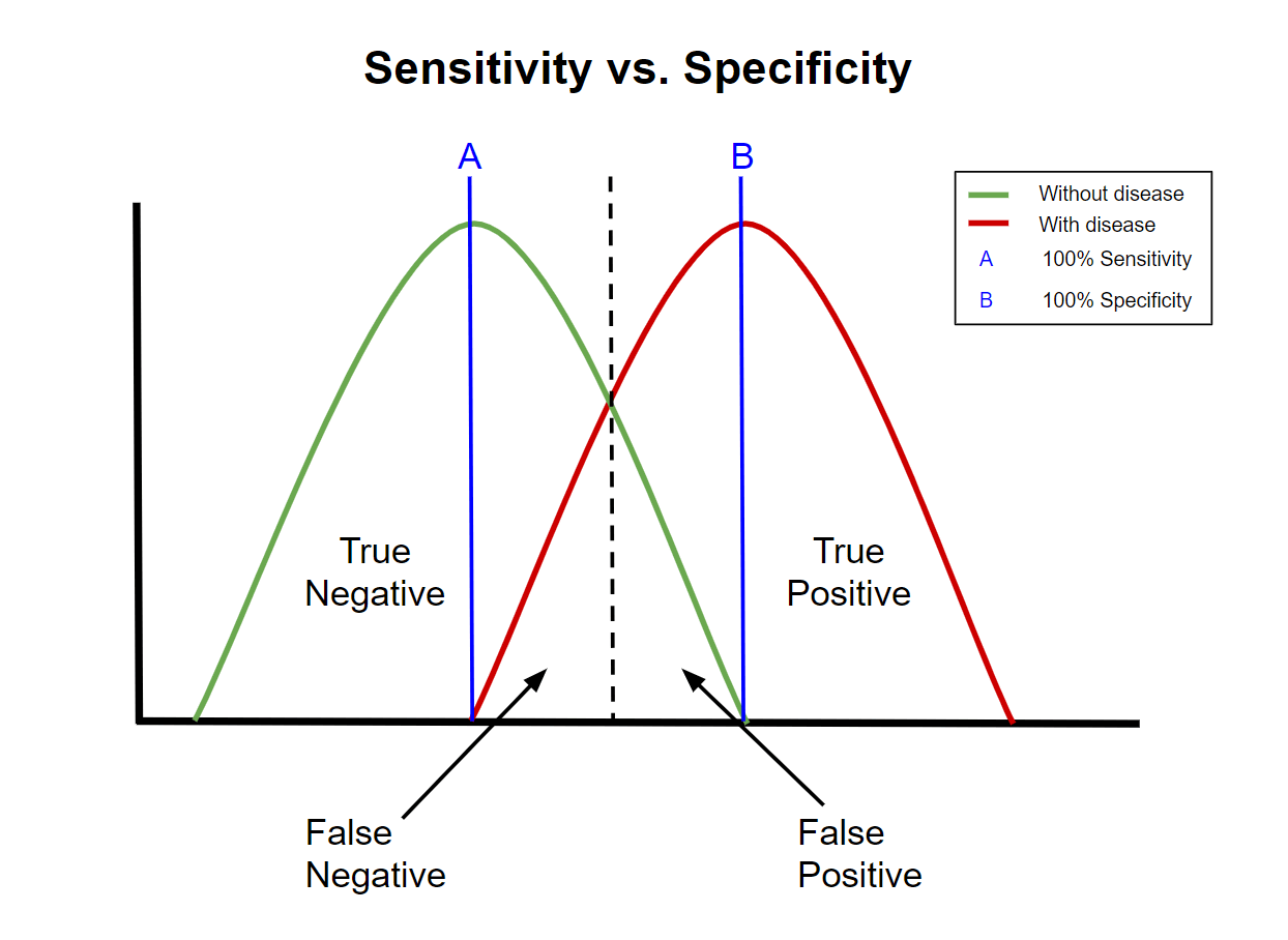
A test with high sensitivity has few false negatives, so a NEGATIVE result reliably rules the disease OUT: SnNout. High-sensitivity tests are the screening/'safety-net' tests you want negative.
A test with high specificity has few false positives, so a POSITIVE result reliably rules the disease IN: SpPin. High-specificity tests are the confirmatory tests you trust when positive.
A meta-analysis of clinical examination for ACL rupture illustrates this perfectly. The Lachman test is the most sensitive of the three (pooled sensitivity 85%, specificity 94%) and is used first, as the test you want negative (SnNout). The pivot-shift test is highly specific (specificity 98%) but insensitive (sensitivity 24%) — so a positive pivot shift effectively rules ACL rupture IN (SpPin), but a negative one does not rule it out. The anterior drawer performs well in chronic injury (sensitivity 92%, specificity 91%) but poorly when acute. Hence the recommendation: perform the Lachman test (to screen) and the pivot shift (to confirm).
One honest qualification, because the numbers reward reading twice. The Lachman is the standard SnNout example, but its specificity (94%) is actually higher than its sensitivity (85%), and its likelihood ratios say the same thing: LR+ around 14 is a large, near-conclusive shift, while LR− of 0.16 is only a moderate one. So the Lachman is in truth the better rule-in test of the two properties, and a negative Lachman lowers the probability of rupture substantially without excluding it — which is exactly why a convincing history with a negative Lachman still earns an MRI. "The more sensitive of the available tests" and "a sensitive test" are not the same claim, and SnNout is a rule of thumb about relative strengths, not a licence to discharge.
For a test read on a continuous scale, moving the cut-off trades sensitivity against specificity: lowering the threshold catches more true positives (higher sensitivity) but creates more false positives (lower specificity), and vice versa. There is no free lunch — the ROC curve displays this entire trade-off. The "best" threshold depends on the cost of a missed case versus a false alarm.
Predictive values & prevalence
Sensitivity and specificity are properties of the test; predictive values are properties of the test applied to a particular population. As prevalence (pre-test probability) falls, the pool of truly diseased people shrinks relative to the well, so even a small false-positive rate generates many false positives — and PPV falls (while NPV rises). The identical test therefore has a high PPV in a high-prevalence (specialist clinic) setting and a low PPV in a low-prevalence (population screening) setting. This is the single most important caveat when applying published test data to your own patients.
- Pre-test probability (prevalence)
- Low
- Effect on PPV
- PPV LOW (many false positives)
- Effect on NPV
- NPV high
- Pre-test probability (prevalence)
- Moderate–high
- Effect on PPV
- PPV higher
- Effect on NPV
- NPV lower
- Pre-test probability (prevalence)
- High
- Effect on PPV
- PPV HIGH
- Effect on NPV
- NPV lower
Worked example: the same test in two populations
Take the Lachman test at its published performance - sensitivity 85%, specificity 94% - and apply it unchanged to two different populations.
A. Acute knee clinic, 1,000 patients, prevalence 50% (500 have an ACL rupture)
- ACL rupture
- TP = 425
- No rupture
- FP = 30
- Total
- 455
- ACL rupture
- FN = 75
- No rupture
- TN = 470
- Total
- 545
- ACL rupture
- 500
- No rupture
- 500
- Total
- 1,000
PPV = 425 / 455 = 93%. NPV = 470 / 545 = 86%.
B. Screening an unselected population, 10,000 people, prevalence 2% (200 have a rupture)
- ACL rupture
- TP = 170
- No rupture
- FP = 588
- Total
- 758
- ACL rupture
- FN = 30
- No rupture
- TN = 9,212
- Total
- 9,242
- ACL rupture
- 200
- No rupture
- 9,800
- Total
- 10,000
PPV = 170 / 758 = 22%. NPV = 9,212 / 9,242 = 99.7%.
The same test, with identical sensitivity and specificity, has a positive predictive value of 93% in one setting and 22% in the other. In the low-prevalence population more than three-quarters of positive results are false, and the reason is visible in the tables: the 6% false-positive rate is applied to 9,800 well people and generates 588 false positives, swamping the 170 true ones. No improvement in the test fixes this - only testing a population in which the disease is actually likely.
Now notice what did not change. LR+ = 0.85 / 0.06 = 14.2 in both tables (425/500 divided by 30/500, and 170/200 divided by 588/9,800 - the same number). That is what "prevalence-independent" means, and it is why likelihood ratios travel between settings when predictive values cannot. Applying it the other way round: pre-test probability 2% gives pre-test odds of 0.0204; multiplied by 14.2 that is post-test odds of 0.289, which converts back to a post-test probability of 22% - exactly the PPV computed from the table, as it must be.
If you are asked why a screening test "does not work" despite excellent published figures, this table is the answer, and it is worth being able to build it in under a minute. Assume a round population, split it by prevalence, apply sensitivity down the diseased column and specificity down the well column, then read PPV across the positive row. The trap in the question is almost always that prevalence has been changed while the test has stayed the same.
Likelihood ratios & post-test probability
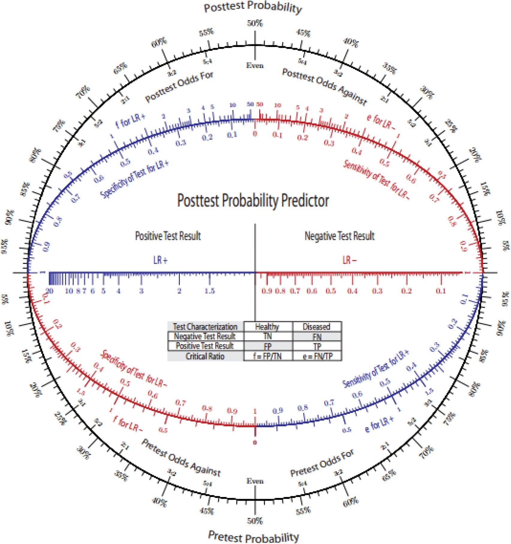
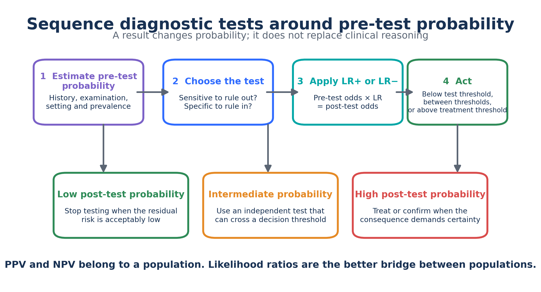
Likelihood ratios (LRs) combine sensitivity and specificity into a single number that tells you how much a given result changes the odds of disease — and, unlike predictive values, they are independent of prevalence:
- LR+ = sensitivity / (1 − specificity) — how much MORE likely a positive result is in disease than in health.
- LR− = (1 − sensitivity) / specificity — how much LESS likely a negative result makes disease.
Apply them as: pre-test odds × LR = post-test odds (convert probability to odds, multiply, convert back; a Fagan nomogram does this graphically).
- LR−
- Less than 0.1
- Effect on probability of disease
- Large, often conclusive change
- LR−
- 0.1 to 0.2
- Effect on probability of disease
- Moderate change
- LR−
- 0.2 to 0.5
- Effect on probability of disease
- Small change
- LR−
- 0.5 to 1
- Effect on probability of disease
- Minimal / rarely important change
- LR−
- 1
- Effect on probability of disease
- No change (test useless at that result)
Using the Lachman data (sensitivity 85%, specificity 94%): LR+ = 0.85 / (1 − 0.94) = 0.85 / 0.06 ≈ 14 (a positive Lachman strongly raises the probability of ACL rupture), and LR− = (1 − 0.85) / 0.94 = 0.15 / 0.94 ≈ 0.16 (a negative Lachman meaningfully lowers it). The high LR+ explains why a positive Lachman is so persuasive.
The ROC curve & AUC
For a test measured on a continuous (or ordinal) scale, the ROC curve plots sensitivity (true positive rate) on the y-axis against 1 − specificity (false positive rate) on the x-axis as the threshold is varied across its full range. A test with no discriminating ability follows the diagonal (line of chance); a good test bows toward the top-left corner. The area under the curve (AUC) summarises overall discrimination in a single number.
- Discrimination
- No better than chance
- Discrimination
- Acceptable
- Discrimination
- Excellent
- Discrimination
- Outstanding
- Discrimination
- Perfect separation
The ROC curve makes the threshold-independent performance of a test visible and lets you compare two tests (the larger AUC discriminates better overall) and choose an operating point that balances the costs of false negatives and false positives for your clinical question.
Overall accuracy = (TP + TN) / N is the most intuitive summary but is misleading in imbalanced populations - the accuracy paradox: in low-prevalence disease a test (or a clinician) that simply calls everyone negative scores a high accuracy yet is clinically useless. That is exactly why sensitivity, specificity and likelihood ratios are preferred over raw accuracy. To pick the operating point, the Youden index (J = sensitivity + specificity − 1, ranging 0 for a useless test to 1 for a perfect one) identifies the optimal ROC threshold - the point that maximises Sn + Sp, i.e. the point on the curve furthest above the chance diagonal - when false positives and false negatives are weighted equally. Shift the chosen point away from the Youden optimum when the costs are asymmetric (favour sensitivity when missing the disease is dangerous).
Agreement & reliability: kappa, ICC and Bland-Altman
Everything above compares a test against a reference standard - that is accuracy, or validity. A separate question is whether two observers, or the same observer twice, get the same answer at all - that is reliability. A classification can be perfectly reproducible and still meaningless, or highly meaningful and hopelessly irreproducible. Every orthopaedic classification paper reports reliability, and "how reproducible is that classification?" is a standard viva question, so the statistics below are examined as often as sensitivity and specificity.
Why raw percentage agreement is not enough. If two surgeons independently classify 100 fractures and agree on 80, that sounds convincing - but if 90% of the fractures are of one type, they would have agreed on roughly 80 by guessing alone. Cohen's kappa corrects observed agreement for the agreement expected by chance:
kappa = (observed agreement − expected agreement) / (1 − expected agreement)
A kappa of 0 means agreement no better than chance; 1 means perfect agreement; negative values mean worse than chance.
- Strength of agreement
- Poor - worse than chance
- Strength of agreement
- Slight
- Strength of agreement
- Fair
- Strength of agreement
- Moderate
- Strength of agreement
- Substantial
- Strength of agreement
- Almost perfect
The variants you must name correctly:
- Inter-observer (inter-rater) reliability - different observers, same images. This is what limits a classification in real multi-surgeon practice.
- Intra-observer (intra-rater) reliability - the same observer, same images, on two separate occasions, far enough apart to prevent recall. Intra-observer agreement is almost always higher than inter-observer, so a paper quoting only the former is flattering its classification.
- Weighted kappa - for ordinal categories, where disagreements are not equally wrong. Calling a Garden III a Garden IV is a smaller error than calling it a Garden I, and weighted kappa credits near-misses. Use it whenever the categories have a natural order.
- Intraclass correlation coefficient (ICC) - the equivalent for continuous measurements (an angle, a length, a score), and for more than two raters.
- Fleiss' kappa - for more than two raters with categorical data.
Kappa is sensitive to the distribution of categories. When one category dominates - most scaphoid radiographs are normal, most slipped epiphyses are stable - the chance-expected agreement is already very high, so even excellent observed agreement leaves little room above chance and kappa can be startlingly low despite 90%+ raw agreement. This is the prevalence effect, and there is a matching bias effect when raters use categories at different overall rates. The practical consequence: never interpret a kappa without knowing the distribution of the categories, and be suspicious of a low kappa reported alongside a high raw agreement - it may be an artefact rather than genuine disagreement.
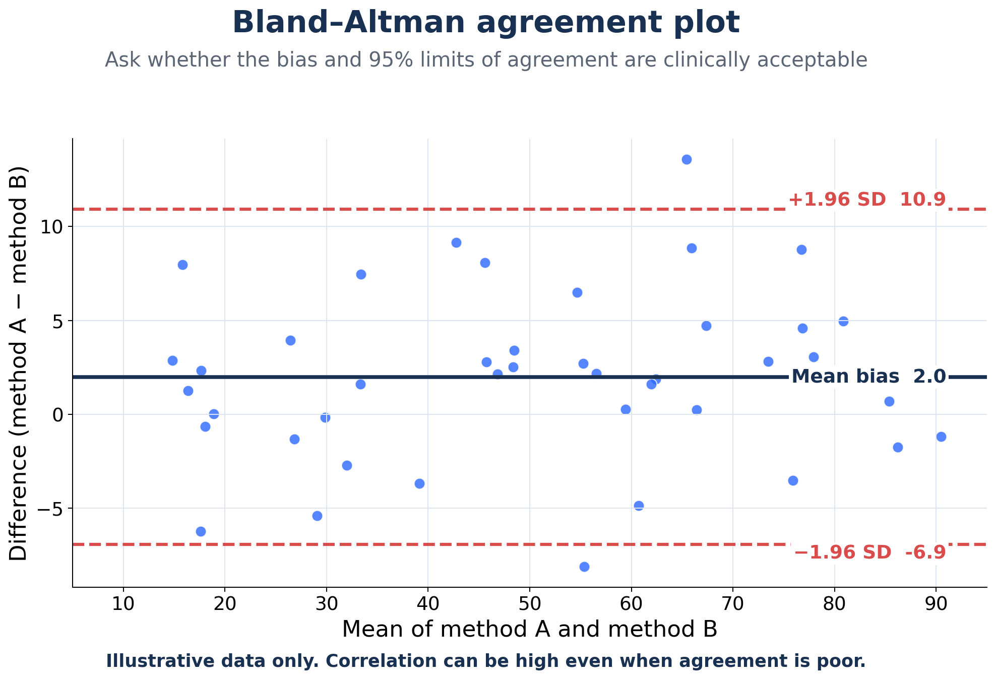
Comparing two ways of measuring the same thing - and the correlation trap. If you want to know whether a new goniometer, navigation system or radiographic method agrees with an established one, a correlation coefficient is the wrong analysis. Two methods can correlate almost perfectly while one reads 10 degrees higher than the other every single time - correlation measures whether they move together, not whether they agree. The correct analysis is a Bland-Altman plot: plot the difference between the two methods against their mean, then report the bias (the mean difference, a systematic offset) and the limits of agreement (bias ± 1.96 SD of the differences). You then judge clinically whether errors that large would change a decision. "They correlated well, r = 0.95" is not evidence of agreement, and saying so is a reliable way to lose a mark.
Why published accuracy is usually too good
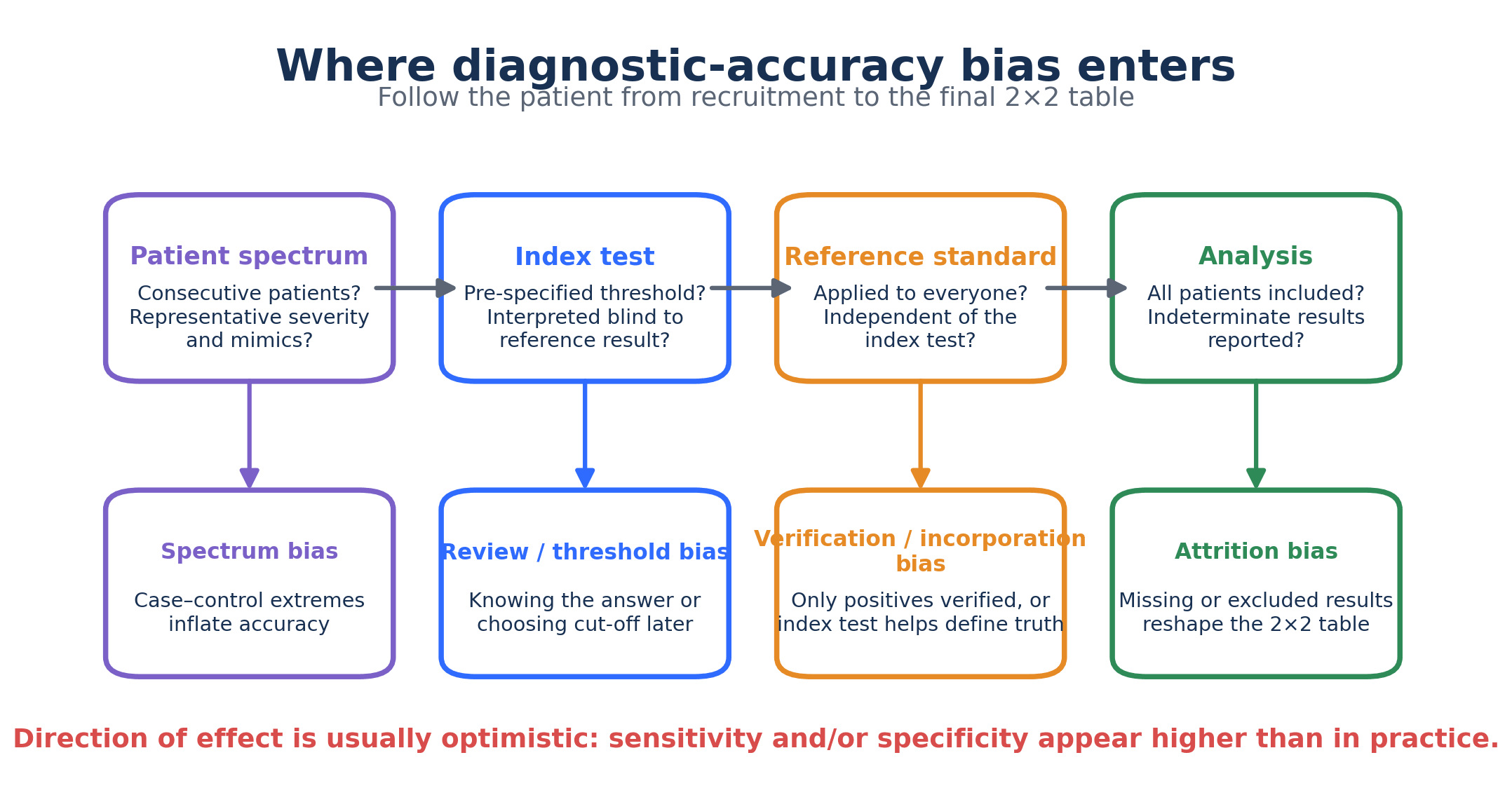
Sensitivity and specificity are called intrinsic test properties, and for teaching purposes that is a useful simplification - but the figures you read are estimates from a study design, and several common flaws push them upwards. Being able to name these is what separates quoting a number from appraising it.
- Spectrum bias - the test is evaluated in florid, advanced cases against healthy volunteers, rather than in the ambiguous patients in whom you would actually use it. Sensitivity looks superb because the disease is obvious. This is why sensitivity and specificity are only "largely" prevalence-independent: change the case mix and they genuinely move.
- Verification (work-up) bias - only patients with a positive index test go on to receive the reference standard, because it is invasive. The false negatives are never counted, so sensitivity is overestimated. Endemic in surgical series where arthroscopy is the reference standard and nobody arthroscopes a normal-looking knee.
- Incorporation bias - the index test is itself part of the reference standard, or contributes to it. The test is then partly being compared against itself, and accuracy is inflated. Common when the "reference" is a clinical diagnosis made by a panel that saw the test result.
- Review bias - the person interpreting the index test knows the reference result, or vice versa. Blinding in both directions is required.
- Design effect - a case-control design (known cases versus known controls) systematically overstates accuracy compared with a consecutive cohort of patients with the relevant clinical presentation, which is the design you should demand.
- Selective and incomplete reporting - the cut-point that maximised accuracy in this dataset is reported as though it had been specified in advance, which overfits it to the sample.
The two acronyms to quote: STARD is the reporting standard for diagnostic accuracy studies (what a paper must state), and QUADAS-2 is the quality appraisal tool used in systematic reviews (how a paper is judged for risk of bias). Naming the right one for the right purpose is a cheap mark.
Diagnostic odds ratio. A single summary of discrimination: DOR = LR+ / LR−, equivalently (TP x TN)/(FP x FN). It is prevalence-independent and convenient for meta-analysis, but it collapses sensitivity and specificity into one figure and so cannot tell you whether a test is better at ruling in or ruling out - which is usually the clinically important question. Quote it as a summary, then give the LRs.
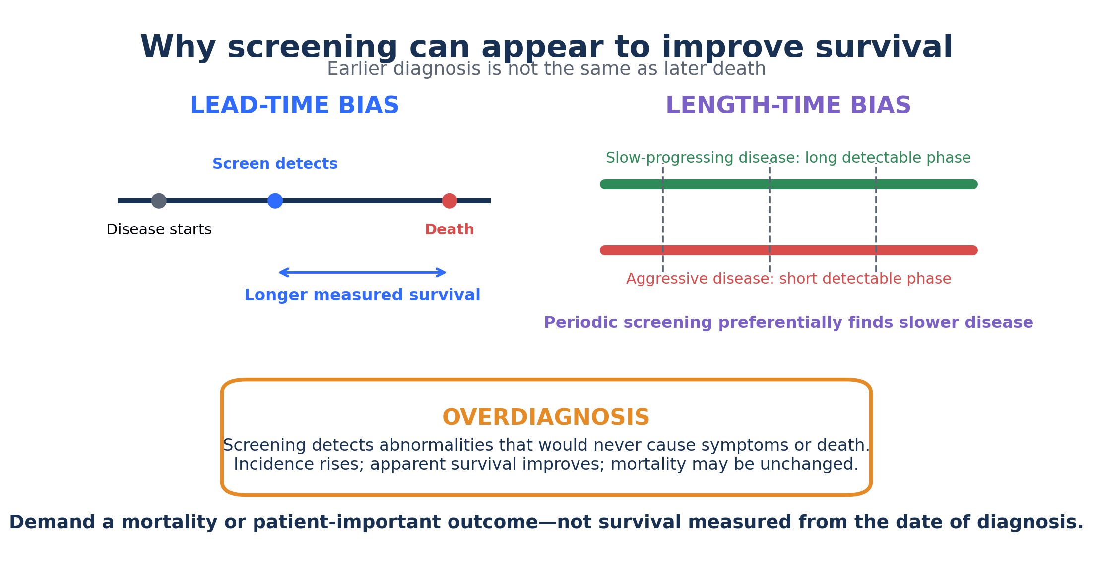
Screening claims are judged on survival, and three biases can manufacture an apparent survival benefit where none exists:
- Lead-time bias - screening advances the moment of diagnosis without postponing death, so survival measured from diagnosis lengthens while the date of death is unchanged.
- Length-time bias - slowly progressive, indolent disease spends longer in a detectable preclinical phase and is therefore preferentially caught by screening, so the screened group is enriched with better-behaved disease.
- Overdiagnosis - the extreme of length-time bias: detection of disease that would never have caused symptoms in the patient's lifetime. Every such case is counted as a screening success and a survivor, while the patient is exposed to the harms of treatment.
The defence against all three is the same: judge screening on disease-specific and all-cause mortality in a randomised comparison, never on survival from diagnosis, five-year survival, or stage shift.
Clinical Relevance: applying the numbers at the bedside
These statistics are not an academic exercise - they change how you choose, sequence and interpret the tests you use every day.
- The statistic that answers it
- A highly SENSITIVE test, when negative (SnNout)
- Orthopaedic example
- Lachman (sens 85%) to screen for ACL rupture; Ottawa ankle rules to exclude fracture
- The statistic that answers it
- A highly SPECIFIC test, when positive (SpPin)
- Orthopaedic example
- Pivot shift (spec 98%) to confirm ACL rupture
- The statistic that answers it
- PPV/NPV - but adjust for the patient's prevalence/pre-test probability
- Orthopaedic example
- A positive screening test in a low-risk clinic has a far lower PPV than in a specialist referral
- The statistic that answers it
- Likelihood ratios (prevalence-independent); pre-test odds x LR
- Orthopaedic example
- A positive Lachman (LR+ ~14) is near-conclusive; a borderline sign (LR ~1) is not
- The statistic that answers it
- ROC / AUC and choice of operating point
- Orthopaedic example
- Comparing an MRI sequence or a clinical sign by AUC
Sequence tests deliberately: screen with a sensitive test (you want a negative to be trustworthy), then confirm with a specific test (you want a positive to be trustworthy). Always anchor on the pre-test probability of the patient in front of you - the same positive result means different things in a 5%-prevalence and a 60%-prevalence population. Quote likelihood ratios rather than a borrowed PPV when you can, because they travel between populations.
A sophisticated caveat: sensitivity and specificity are "intrinsic" but not immutable - they shift with the spectrum of patients studied (spectrum bias). Sensitivity looks higher when the diseased group is severe/advanced, and specificity looks higher when the non-diseased controls are clearly well rather than symptomatic mimics - so a test validated in a tertiary cohort can underperform in primary care. Published estimates are further threatened by verification (work-up) bias - applying the gold standard only to test-positives inflates sensitivity and deflates specificity - by an imperfect or absent reference standard, and by review bias when the index and reference tests are interpreted with knowledge of each other. The standard tool for appraising these risks in a diagnostic-accuracy study is QUADAS-2 (patient selection, index test, reference standard, flow and timing). So before transplanting a study's numbers to your patient, check that its spectrum and methodology resemble your setting.
Mnemonics & Memory Aids
- Build the 2×2 (rows = test result, columns = true disease status; TP/FP/FN/TN).
- Sn = TP/(TP+FN), Sp = TN/(TN+FP) — down the columns, prevalence-independent.
- PPV = TP/(TP+FP), NPV = TN/(TN+FN) — across the rows, prevalence-DEPENDENT (PPV falls as prevalence falls).
- SnNout / SpPin — sensitive+negative rules out; specific+positive rules in.
- LR+ = Sn/(1−Sp), LR− = (1−Sn)/Sp — prevalence-independent; pre-test odds × LR = post-test odds.
- ROC = Sn vs 1−Sp across thresholds; AUC 0.5 chance → 1.0 perfect.
SnNout / SpPinThe two rules
Hook:SnNout and SpPin: sensitive-negative rules out, specific-positive rules in.
COLUMNSReading the table
Hook:Read sensitivity/specificity down the COLUMNS, predictive values across the rows.
Viva practice
Viva practice
Practise clinical reasoning and management decisions out loud
“Draw a 2x2 table for a diagnostic test against a gold standard and define sensitivity, specificity, and the positive and negative predictive values. Which depend on prevalence?”
“What is a likelihood ratio, why is it useful, and what is a ROC curve?”
“You quote a fracture classification in a viva. The examiner asks: how reproducible is it, how would you measure that, and what would make you distrust a published reliability figure?”
Exam cheat sheet
From the 2×2 table
- Sensitivity = TP/(TP+FN); Specificity = TN/(TN+FP) - down the columns, prevalence-independent
- PPV = TP/(TP+FP); NPV = TN/(TN+FN) - across the rows, prevalence-DEPENDENT
- SnNout: sensitive + negative rules OUT; SpPin: specific + positive rules IN
Predictive values
- Answer the patient's question but depend on prevalence (pre-test probability)
- Low prevalence (screening) → low PPV, high NPV
- High prevalence (specialist) → high PPV
Likelihood ratios
- LR+ = Sn/(1-Sp); LR- = (1-Sn)/Sp; prevalence-independent
- Pre-test odds x LR = post-test odds (Fagan nomogram)
- LR+ over 10 or LR- under 0.1 = large, often conclusive change
ROC / AUC
- ROC = sensitivity vs (1 - specificity) across thresholds
- Good test bows to top-left; diagonal = chance
- AUC 0.5 chance, 0.8-0.9 excellent, 1.0 perfect; compare tests by AUC
Agreement & reliability
- Accuracy = agreement with a reference standard; reliability = agreement between observers. Different questions
- Cohen's kappa corrects raw agreement for chance. Landis & Koch: 0.21-0.40 fair, 0.41-0.60 moderate, 0.61-0.80 substantial, over 0.81 almost perfect
- Weighted kappa for ORDINAL grades (near-misses count for less); ICC for continuous measures; Fleiss for over 2 raters
- Intra-observer agreement always beats inter-observer - a paper quoting only intra-observer is flattering itself
- Kappa paradox: with one dominant category, chance agreement is high, so kappa can be low despite over 90% raw agreement
- Agreement between two MEASUREMENT methods = Bland-Altman (bias and limits of agreement), NEVER a correlation coefficient
Appraising the study
- Spectrum bias: florid cases vs healthy volunteers inflates sensitivity - the reason Sn/Sp are only LARGELY prevalence-independent
- Verification (work-up) bias: only test-positives get the reference standard, so false negatives are never counted - sensitivity overestimated
- Incorporation bias: index test forms part of the reference standard - the test is compared with itself
- Review bias: unblinded interpretation. Case-control design overstates accuracy versus a consecutive cohort
- STARD = reporting standard; QUADAS-2 = quality/risk-of-bias appraisal. Do not swap them
- Diagnostic odds ratio = LR+/LR-; prevalence-independent but hides whether a test rules in or out
- Screening claims: lead-time, length-time and overdiagnosis all fake a survival benefit - demand randomised MORTALITY data, not survival from diagnosis
Evidence Base
Clinical diagnosis of an anterior cruciate ligament rupture: a meta-analysis
- Pooled across 28 studies: the Lachman test had sensitivity 85% (95% CI 83-87) and specificity 94% (92-95) - a strong screening test (SnNout).
- The pivot-shift test was highly specific (98%, 96-99) but insensitive (24%, 21-27) - a confirmatory test (SpPin); the anterior drawer performed well in chronic (92%/91%) but not acute injury.
- Recommends performing both the Lachman (to screen) and the pivot shift (to confirm) - the SnNout/SpPin principle in practice.
Diagnostic tests 4: likelihood ratios
- Standard methodological reference defining the likelihood ratio and how it links pre-test and post-test probability.
- LR+ = sensitivity / (1 - specificity); LR- = (1 - sensitivity) / specificity; applied as pre-test odds x LR = post-test odds.
- Likelihood ratios are independent of prevalence - their key advantage over predictive values - and can be applied with a Fagan nomogram.
Determining Risk of Falls in Community Dwelling Older Adults: A Systematic Review and Meta-analysis Using Posttest Probability
- Calculated sensitivity, specificity, likelihood ratios and post-test probability for many fall-risk measures - a worked demonstration of applying these statistics to real clinical tests.
- No single test had strong post-test probability; cumulative (combined) measures performed better - illustrating how likelihood ratios chain from pre-test to post-test probability.
- The best-supported functional measures were the Timed Up and Go (12 s or more), the Berg Balance Scale (50 or less) and the 5-times sit-to-stand (12 s or more).
The orthopaedic test-performance figures used as worked examples (Lachman, pivot shift, anterior drawer) come from Benjaminse et al. 2006 (DOI); the likelihood-ratio method from Deeks & Altman 2004 (DOI); a worked likelihood-ratio/post-test-probability application from Lusardi et al. 2017 (DOI); the kappa bands from Landis & Koch 1977; and the method for comparing two measurement techniques from Bland & Altman 1986. The formulas and definitions are standard biostatistics presented as mathematical relationships rather than empirical claims - the arithmetic in the worked 2x2 tables can and should be checked by recomputing it.